Econometric Models

(Updated 6-30-2023)

This post lists common econometric models. It is currently work-in-progress. Please let me know if you have models in mind that I should include.

Table of Contents

• Two-sample t test
• Logistics regression
  • Log-odds
  • Logistic function
  • The odds ratio
• Experiments
  • How to reduce the size of an experiment?
• IV
• Linear regression
  • Clustering standard errors
• ARIMA
• DiD
  • Group-time treatment effect
• ANOVA
• Post-estimation

Two-sample t test

Two-sample t test

Logistics regression

In statistics, the logistic model is a statistical model that models the probability of one event taking place by having the log-odds for the event be a linear combination of one or more independent variables (Reference).

In regression analysis, logistic regression is estimating the parameters of a logistic model.

Formally, in binary logistic regression there is a single binary dependent variable, coded by an indicator variable, where the two values are labeled “0” and “1”, while the independent variables can each be a binary variable or a continuous variable. The corresponding probability of the value labeled “1” can vary between 0 and 1. The function that converts log-odds to probability is the logistic function.

Log-odds

\(ln(\frac{p(x)}{1 - p(x)}) = \beta_0 + \beta_1 x\)

When \(x\) increases by 1, the odds of success increases by \(\beta_1\) percent multiplicatively (Reference).

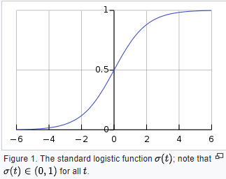
Logistic function

The function that converts log-odds to probability is the logistic function.

Let \(t\) be a linear combination of parameters and independent variable

\[t = \beta_0 + \beta_1 x\]

The logistic function is

\[p(x) = \delta(t) = \frac{1}{1+e^{-(\beta_0+\beta_1x)}}\]

\(p(x)\) is interpreted as the probability of the dependent variable \(Y\) equaling a success rather than a failure.

The odds ratio

For a continuous independent variable the odds ratio can be defined as:

\[OR = e^{\beta_1}\]

This exponential relationship provides an interpretation for \(\beta_1\): the odds multiply by \(e^{\beta_1}\) for every 1-unit increase in x.

Experiments

How to reduce the size of an experiment?

1. Increase practical significance, alpha, or beta
2. Change unit of diversion to a smaller unit
3. Target experiment to specific traffic Reference: Udacity A/B testing course, Lesson 4

IV

• IV overview

• IV vs OLS (Reference here)

• Two-stage least squares (2SLS) (Mostly Harmless 4.6.4)

  • Formula

    Causal model of interest: \(y = \beta x + \eta\)

    First stage equation: \(x = Z\pi + \varepsilon\)

  • Implementation in Python https://bashtage.github.io/linearmodels/iv/examples/basic-examples.html

  • Bias

    \[E[\hat{\beta}_{2SLS} - \beta] \approx \frac{\sigma_{\eta \varepsilon}}{\sigma^2_\varepsilon}\frac{1}{F+1}\]

    where \(F = \frac{E(\pi'Z'Z\pi)/Q}{\sigma^2_\varepsilon}\) and \(Q = E(P_z)\) where \(P_z = Z(Z'Z)^{-1}Z'\).

    • Bias is small when F-stat is large, i.e. if the joint significance of all regressors in the first stage regression is large.

    • Adding weak instruments increases bias by increasing \(Q\) but not \(E(\pi'Z'Z\pi)\) or \(\sigma^2_\varepsilon\).

  • Practical recommendations

    • Report first stage and make sure the magnitude and sign are what I expect.
    • Report F-stats on excluded instruments. Rule of thumb: 10.
    • Report just-identified estimates using single best IV because just-identified IV is median-unbiased.
    • Check overidentified 2SLS estimates with LIML. LIML is less precise than 2SLS but also less biased.
    • Look at coefficients, t-stats, F-stats for excluded instruments in the reduced-form regression of dependent variables on instruments. If you can’t see the causal relation of interest in the reduced form, it’s probably not there.

Linear regression

Clustering standard errors

• For nested models, the most aggregate level matters the most
• Clustering in Stata Clustering in R

ARIMA

ARIMA: Auto Regressive Integrated Moving Average. It explains a given time series based on its own past values (its own lags and the lagged forecast errors), so that equation can be used to forecast future values.

Regression kink design

DiD

de Chaisemartin & D’Haultfoeuille (2020): heterogeneous treatment effects Stata package R package

Group-time treatment effect

Reference: Callaway & Sant’Anna (2020)

To put the above equation into English, it means that for group g at time t, the average treatment effect on the treated is the difference in outcome for this group when they are treated compared to when they are not (the counterfactual outcome).

The above equation applies to time period t for a group that went through treatment in time period g. The coefficient captures the ATT(g, t).

The above equation is the event study formula for each group. the are the anticipation effects, and the are the treatment effects.

The aggregation is done by

where

It first averages across all time periods for each group, and then averages across groups.

Callaway & Sant’Anna (2020) R package

ANOVA

Reference

Post-estimation

There are a lot of post estimation that can be carried out. For example, for xtlogit in stata, postestimation commands can be found here.