Panel data modeling for the Stand Your Ground Law project

The baseline specification is very straightforward. Note that both states and years are binary variables. We have 66 regressors in total here.

The way it is implemented is:

xtset state year
qui xtreg murder law i.year [aweight=popwt], fe vce(cluster state)

Then we added region-by-year fixed effects to control for region-specific time effects. Regions are binary variables. We would like to see how different the time trends are between the baseline trend and each other region’s.

The way to implement it is:

** First, generate region-by-year fixed effects
forvalues j = 2000/2014{
	gen year`j'=(year==`j') # ex: year2000 = 1 if we are in year 2000
	gen r`j'1=year`j'*northeast # ex: r20001 = 1 if we are in year 2000 and in the Northeast
	gen r`j'2=year`j'*midwest
	gen r`j'3=year`j'*south
	gen r`j'4=year`j'*west
	drop year`j'
}

This way, we generate 60 variables that represent 15 years * 4 regions.

Then we put all of them into one global macro:

global region r20001-r20144

Then we add these variables as regressors:

qui xtreg murder law i.year $region [aweight=popwt], fe vce(cluster state)

Here is the structure of the regional data:

Below is how it is in the form of region by year dummies. r20003 for Alabama equals to 1 because it is the year 2000 and Alabama is in the South.

Then we controlled for time-varying factors:

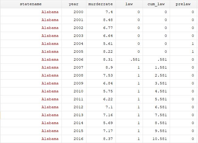
Then we controlled for Ashenfelter’s dip. Namely, if there is an increased amount of murder two years prior to the law passing, the prelaw dummy would be able to capture this effect.

The structure of the prelaw dummy is:

Then we controlled for state-specific trends:

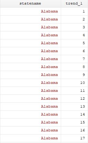
Data related to the state-specific trends. Note that it is the product of a discrete random variable (year) and a binary variable (state_i)